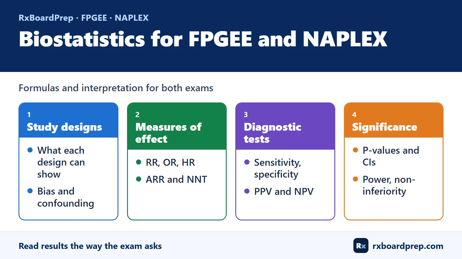
Biostatistics for FPGEE and NAPLEX: Formulas and Interpretation
Biostatistics questions reward a small set of ideas used precisely. You rarely need advanced mathematics; you need to know which measure a study reports, how to calculate it from a few numbers, and what it does and does not mean for a patient. The same core material appears on both pharmacy board exams run by the National Association of Boards of Pharmacy (NABP):
- Foreign Pharmacy Graduate Equivalency Examination (FPGEE): NABP’s FPGEE Content Outline lists “Biostatistics and research methods” (study design, statistical tests, data collection instruments, research ethics) and pharmacoepidemiology within Social, Behavioral and Administrative Sciences, and evidence-based practice within Pharmacy Practice and Clinical Sciences. See our 2026 FPGEE content outline guide.
- North American Pharmacist Licensure Examination (NAPLEX): the NAPLEX Content Outline places biostatistical, epidemiological and pharmacoeconomic measures among the Domain 1 calculations, alongside research design principles and biostatistics (blinding, randomization, biases, statistical tests and outcomes, ethics) and the evaluation of drug information resources. See our 2026 NAPLEX content outline guide.
This guide works through each concept with a short original example. Do the arithmetic yourself before reading the answer.
Study designs and what each can show
| Design | How it works | Typical measure | Main strength | Main limitation |
|---|---|---|---|---|
| Randomized controlled trial (RCT) | Participants randomly assigned to treatment or control, then followed | Relative risk, hazard ratio, mean difference | Randomization balances known and unknown confounders, so it can support cause and effect | Costly; selected populations; may be too short or small for rare harms |
| Prospective cohort | Exposed and unexposed groups followed forward for outcomes | Relative risk, incidence | Establishes that exposure came before outcome | Confounding; loss to follow-up; slow for rare outcomes |
| Retrospective cohort | Uses existing records to compare exposed and unexposed groups | Relative risk, hazard ratio | Faster and cheaper | Depends on record quality; confounding |
| Case-control | Starts with people who have the outcome (cases) and without it (controls), then looks back at exposures | Odds ratio | Efficient for rare outcomes | Recall and selection bias; cannot give incidence |
| Cross-sectional | Measures exposure and outcome at one point in time | Prevalence, prevalence ratio | Quick snapshot | Cannot show which came first |
| Case report or case series | Describes one or a few patients | None (descriptive) | Generates hypotheses, signals rare adverse effects | No comparison group |
| Systematic review and meta-analysis | Systematically finds and combines studies on one question | Pooled effect | Summarizes the totality of evidence | Only as good as the included studies; heterogeneity |
A useful rule: only randomization protects against unknown confounders. Observational designs can adjust for confounders that were measured, but not for those that were not.
Measures of association and effect
Relative risk and odds ratio
Relative risk (RR) = risk of the outcome in the exposed (or treated) group ÷ risk in the unexposed (or control) group. It is used in cohort studies and RCTs, where incidence can be measured.
Odds ratio (OR) = odds of exposure among cases ÷ odds of exposure among controls; equivalently (a × d) ÷ (b × c) in a 2 × 2 table. In a cohort study or trial, the same calculation compares the odds of the outcome in the exposed and unexposed groups. It is the natural measure for case-control studies, where risk cannot be calculated. When the outcome is rare (often taken as under about 10%), the OR approximates the RR.
For both: 1 means no difference; above 1 means higher risk or odds in the exposed group; below 1 means lower.
Example 1. In a cohort study, 60 of 400 patients taking a drug developed a rash, compared with 45 of 600 patients not taking it. Calculate the RR and the OR.
- Risk, exposed = 60 ÷ 400 = 0.15. Risk, unexposed = 45 ÷ 600 = 0.075.
- RR = 0.15 ÷ 0.075 = 2.0. Patients taking the drug had twice the risk of rash.
- OR = (60 × 555) ÷ (340 × 45) = 33,300 ÷ 15,300 = 2.18.
Because a rash was not rare here (15% in the exposed group), the OR overstates the RR. Do not read an OR as if it were a risk ratio when the outcome is common.
Absolute risk reduction, relative risk reduction and NNT
- Absolute risk reduction (ARR) = control event rate (CER) − experimental event rate (EER).
- Relative risk reduction (RRR) = ARR ÷ CER, which also equals 1 − RR.
- Number needed to treat (NNT) = 1 ÷ ARR, with ARR as a decimal, rounded up to the next whole number. Always state the time frame.
Example 2. In a 2-year RCT, a stroke occurred in 80 of 1,000 patients on a new drug and 100 of 1,000 on the control. Calculate RR, ARR, RRR and NNT.
- EER = 80 ÷ 1,000 = 0.08. CER = 100 ÷ 1,000 = 0.10.
- RR = 0.08 ÷ 0.10 = 0.80.
- ARR = 0.10 − 0.08 = 0.02 (2%).
- RRR = 0.02 ÷ 0.10 = 0.20 (20%), which equals 1 − 0.80.
- NNT = 1 ÷ 0.02 = 50. Treating 50 patients for 2 years prevents one stroke.
A “20% reduction” sounds larger than “2 percentage points”, but they describe the same result. Relative measures look impressive when baseline risk is low; absolute measures tell you the size of the benefit for an individual. Exam distractors often swap the two.
Number needed to harm
Number needed to harm (NNH) = 1 ÷ absolute risk increase (ARI), where ARI = adverse event rate on treatment − rate on control.
Example 3. In the same trial, major bleeding occurred in 3.0% of the drug group and 1.5% of the control group. Calculate the NNH.
- ARI = 0.030 − 0.015 = 0.015.
- NNH = 1 ÷ 0.015 = 66.7, reported here as 67 (rounded up) over 2 years.
Rounding conventions for NNH differ between references (some round down to be conservative), so follow any instruction in the question. Putting Examples 2 and 3 together: for every 50 patients treated for 2 years, one stroke is prevented; for every 67, one major bleed is caused. That trade-off is the clinically useful answer.
Hazard ratio
A hazard ratio (HR) compares the instantaneous rate of an event over time between two groups, usually from a time-to-event (survival) analysis such as Cox regression. An HR of 0.75 means that, at any point during follow-up, the treated group had a 25% lower rate of the event than the control group. It assumes the ratio is roughly constant over time (the proportional hazards assumption). An HR is not a ratio of cumulative risks and cannot be turned directly into an NNT without event rates at a stated time point.
Diagnostic tests: sensitivity, specificity, PPV and NPV
Using a 2 × 2 table of true positives (TP), false positives (FP), false negatives (FN) and true negatives (TN):
- Sensitivity = TP ÷ (TP + FN): the proportion of people with the disease who test positive. A highly sensitive test, when negative, helps rule a disease out.
- Specificity = TN ÷ (TN + FP): the proportion of people without the disease who test negative. A highly specific test, when positive, helps rule a disease in.
- Positive predictive value (PPV) = TP ÷ (TP + FP): the probability that a positive result is a true positive.
- Negative predictive value (NPV) = TN ÷ (TN + FN): the probability that a negative result is a true negative.
Sensitivity and specificity are properties of the test. PPV and NPV also depend on how common the disease is (prevalence).
Example 4. A screening test has 90% sensitivity and 80% specificity. It is used in 1,000 people where the prevalence is 10%. Calculate the PPV and NPV. Then repeat at a prevalence of 40%.
At 10% prevalence: 100 have the disease and 900 do not.
- TP = 0.90 × 100 = 90; FN = 10. TN = 0.80 × 900 = 720; FP = 180.
- PPV = 90 ÷ (90 + 180) = 33.3%. NPV = 720 ÷ (720 + 10) = 98.6%.
At 40% prevalence: 400 have the disease and 600 do not.
- TP = 360; FN = 40. TN = 480; FP = 120.
- PPV = 360 ÷ 480 = 75%. NPV = 480 ÷ 520 = 92.3%.
The same test gives very different predictive values in different populations. In a low-prevalence setting, most positive results from a moderately specific test are false positives.
P-values and confidence intervals
A p-value is the probability of observing a result at least as extreme as the one seen, assuming the null hypothesis (no difference) is true. If p is below the pre-set significance level (alpha, usually 0.05), the result is called statistically significant. A p-value does not give the probability that the null hypothesis is true, and it says nothing about the size or clinical importance of an effect.
A 95% confidence interval (CI) gives a range of values compatible with the data; it shows both the size of the effect and its precision. The quick significance check:
- For ratios (RR, OR, HR), the line of no effect is 1. If the 95% CI excludes 1, the result is significant at p < 0.05 (two-sided).
- For differences (mean difference, ARR), the line of no effect is 0. If the 95% CI excludes 0, the result is significant.
Example 5. Which of these results are statistically significant at the 0.05 level?
| Result | Significant? | Why |
|---|---|---|
| HR 0.82 (95% CI 0.70 to 0.96) | Yes | The CI excludes 1; an 18% lower hazard, plausibly 4% to 30% |
| RR 0.90 (95% CI 0.78 to 1.04) | No | The CI includes 1 |
| Mean difference in systolic blood pressure −4 mm Hg (95% CI −7 to −1) | Yes | The CI excludes 0 |
“Not statistically significant” does not prove that two treatments are equal. The second result is compatible with anything from a 22% benefit to a 4% harm; the study may simply have been too small.
Statistical vs clinical significance. A very large trial can find a p-value below 0.001 for a 1 mm Hg blood pressure difference that no patient would notice. Always ask whether the size of the effect matters.
Type I and type II errors, and power
| Truly no difference | Truly a difference | |
|---|---|---|
| Study finds a difference | Type I error (false positive), probability = alpha | Correct |
| Study finds no difference | Correct | Type II error (false negative), probability = beta |
- Alpha is usually set at 0.05.
- Power = 1 − beta: the probability of detecting a true difference of a given size. Trials are commonly designed for 80% or 90% power, meaning a 20% or 10% chance of missing a true effect of the size they planned for.
- Power increases with a larger sample size, a larger true effect, less variability, and a higher alpha.
Exam pattern: a small trial reports “no significant difference”. The concern is a type II error from inadequate power, not a type I error.
Non-inferiority trials
A non-inferiority trial asks whether a new treatment is not worse than an active comparator by more than a pre-specified non-inferiority margin. Researchers choose it when a new drug may offer other advantages (fewer adverse effects, easier dosing, lower cost) and a placebo control would be unethical.
Example 6. A trial compares a new anticoagulant with a standard one for stroke prevention. The pre-specified non-inferiority margin is an HR of 1.30 (the upper limit of the 95% CI must fall below 1.30). Interpret each result.
- HR 1.08 (95% CI 0.92 to 1.27): the upper limit is below 1.30, so non-inferiority is shown. The CI includes 1, so superiority is not shown.
- HR 0.85 (95% CI 0.74 to 0.97): the upper limit is below 1.30 and below 1, so the new drug is non-inferior and, if superiority testing was pre-specified, also superior.
- HR 1.12 (95% CI 0.96 to 1.35): the upper limit crosses 1.30, so non-inferiority is not shown. This does not prove the new drug is inferior; the result is inconclusive.
In non-inferiority trials, a per-protocol analysis is usually examined alongside intention-to-treat, because an intention-to-treat analysis can make two treatments look more similar than they are.
Intention-to-treat vs per-protocol
- Intention-to-treat (ITT): analyze every participant in the group they were randomized to, whether or not they took the treatment as assigned. This preserves the balance created by randomization and reflects real-world use. It is the standard primary analysis for superiority trials.
- Per-protocol (PP): analyze only participants who followed the protocol closely enough. It estimates the effect when the treatment is taken as intended, but it can reintroduce bias, because the people who adhere may differ from those who do not.
- Modified ITT usually excludes a defined group (for example, randomized participants who never received a dose). Check how the authors define it.
Multiplicity
Every additional comparison raises the chance of a false-positive result.
Example 7. A study tests 10 independent secondary outcomes, each at alpha = 0.05, and the treatment truly has no effect on any of them. What is the probability of at least one “significant” result by chance?
- Probability of no false positives = 0.95 to the power of 10 = 0.599.
- Probability of at least one = 1 − 0.599 = 0.40, or about 40%.
- A Bonferroni correction would test each outcome at 0.05 ÷ 10 = 0.005.
This is why the primary endpoint carries the main conclusion, why secondary and subgroup findings are usually treated as hypothesis-generating, and why trials pre-specify their analyses. A subgroup that “worked” when the overall trial did not is a classic trap.
Common interpretation traps
- Reading relative risk reduction as absolute benefit. A 50% RRR can be a 1-percentage-point ARR.
- Treating an odds ratio as a relative risk when the outcome is common.
- Calling “not significant” proof of no difference. Check the CI and the power.
- Assuming p < 0.05 means a clinically important effect. Look at the size of the effect.
- Reporting NNT without a time frame. An NNT of 50 over 2 years differs from 50 over 6 months.
- Using the wrong line of no effect: 1 for ratios, 0 for differences.
- Assuming PPV transfers between populations. It falls as prevalence falls.
- Confusing association with causation in observational studies.
- Over-reading subgroup and secondary results when many comparisons were made.
Put it into practice
Biostatistics improves fastest with short, frequent practice: a few calculations and one interpretation question several times a week, mixed in with your other topics. For the formulas used elsewhere in pharmacy calculations, see our NAPLEX calculation formulas guide. To test yourself under time pressure, the free timed FPGEE sets and NAPLEX mock exams on our Free Practice Exams page include biostatistics alongside clinical and calculation questions, with no account needed. If you are preparing for the FPGEE and want guided teaching across all four domains, see RxBoardPrep FPGEE Prep.
References
- National Association of Boards of Pharmacy. FPGEE Content Outline (2025). https://nabp.pharmacy/wp-content/uploads/2025/10/FPGEE-Content-Outline.pdf. Accessed 28 October 2026.
- National Association of Boards of Pharmacy. NAPLEX Content Outline (effective for examinations beginning 1 May 2025), Domain 1, sections C.8, E and F. https://nabp.pharmacy/wp-content/uploads/NAPLEX-Content-Outline.pdf. Accessed 28 October 2026.
- Laupacis A, Sackett DL, Roberts RS. An assessment of clinically useful measures of the consequences of treatment. N Engl J Med. 1988;318(26):1728-1733. https://doi.org/10.1056/NEJM198806303182605.
- Altman DG, Bland JM. Diagnostic tests 2: predictive values. BMJ. 1994;309(6947):102. https://doi.org/10.1136/bmj.309.6947.102.
- US Food and Drug Administration. Non-Inferiority Clinical Trials to Establish Effectiveness: Guidance for Industry. November 2016. https://www.fda.gov/regulatory-information/search-fda-guidance-documents/non-inferiority-clinical-trials.
- US Food and Drug Administration. Multiple Endpoints in Clinical Trials: Guidance for Industry. October 2022. https://www.fda.gov/regulatory-information/search-fda-guidance-documents/multiple-endpoints-clinical-trials.
- International Council for Harmonisation. E9 Statistical Principles for Clinical Trials (1998) and E9(R1) Addendum on Estimands and Sensitivity Analysis (2019). https://www.ich.org/page/efficacy-guidelines.
- Moher D, Hopewell S, Schulz KF, et al. CONSORT 2010 explanation and elaboration: updated guidelines for reporting parallel group randomised trials. BMJ. 2010;340:c869. https://doi.org/10.1136/bmj.c869.
RxBoardPrep is an independent education provider and is not affiliated with or endorsed by NABP.
How this guide was prepared: drafted with AI assistance from the sources listed above, fact-checked against those sources, with every calculation independently recomputed before publication. Published by RxBoardPrep under the editorial oversight of Talha Shafique, PharmD, MPH.